



How to Improve Disease Biomarker Discovery Antibody Analysis Optimization in Research Workflows
Quick Answer
A research team can improve disease biomarker discovery antibody analysis optimization by troubleshooting in a strict sequence: confirm sample comparability, verify antibody specificity, test assay performance under the actual sample matrix, and then revisit normalization, thresholding, and hit ranking. If candidate biomarkers still show inconsistent behavior after those checks, the next step is usually not to repeat the same assay at larger scale. It is to move the most defensible candidates into orthogonal validation. This sequence helps separate biological variability from technical variability, improves data interpretation, and reduces the risk of advancing artifacts that later fail result validation.
Why Antibody-Analysis Bottlenecks Slow Biomarker Discovery
In many translational assay workflows, the core problem is not a complete lack of signal. The problem is that the signal is too unstable, too weak, or too context-dependent to support the next decision. A candidate biomarker may look convincing in one cohort, weaken in another, vary across replicates, or lose support when measured by a different protein-level verification method.
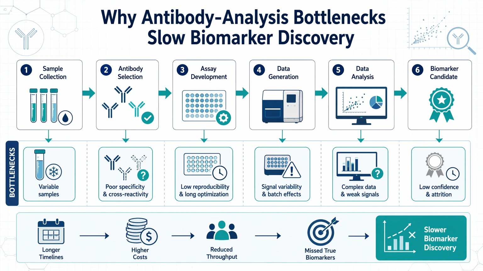
This loss of confidence usually appears at the boundary between biology and measurement. Disease samples are heterogeneous. Antibodies detect epitopes rather than abstract protein names. Sample matrices can suppress or distort signal. Assays can compress weak responses near the lower end of their analytical range. Normalization rules may change hit ranking more than expected. When several of these issues overlap, teams can end up debating the data without knowing whether the real problem is the sample, the reagent, the assay, or the interpretation strategy.
For disease biomarker discovery, antibody analysis is therefore a workflow optimization problem rather than a single-assay problem. The practical goal is to identify where confidence declines, what type of error is most plausible, and which corrective step is most likely to improve validation readiness before more samples and budget are committed.
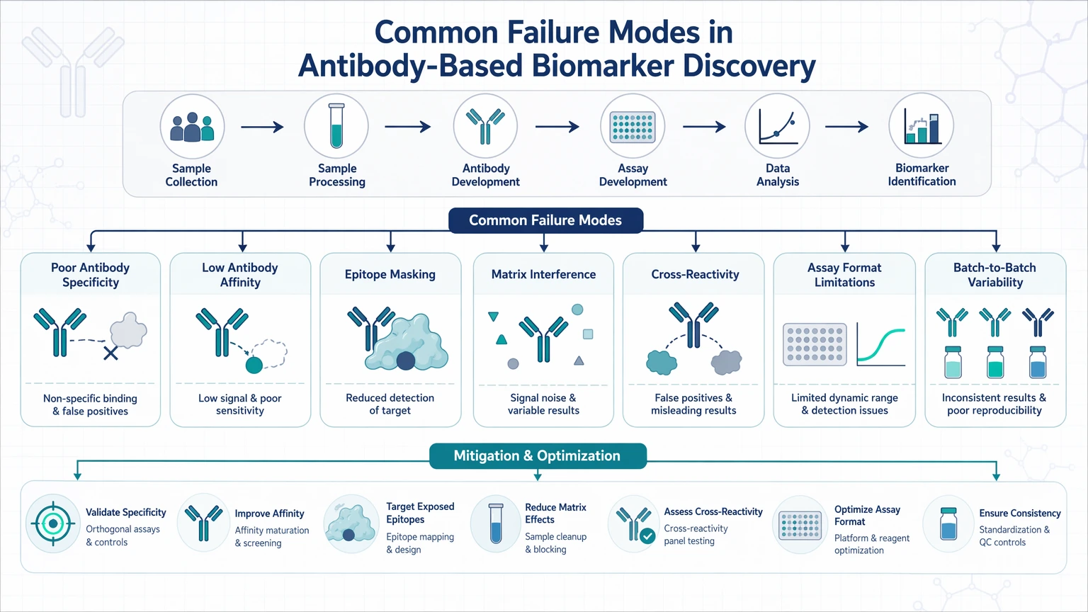
Common Failure Modes in Antibody-Based Biomarker Discovery
Sample-driven failure modes
Sample-related problems often look like weak or inconsistent biology, but the distortion may begin well before measurement.
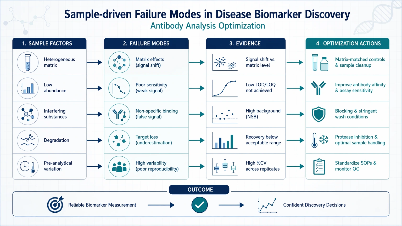
Common examples include:
- uneven sample input consistency across cohorts or plates
- degradation caused by collection, storage, or freeze-thaw history
- disease-state heterogeneity that changes apparent biomarker abundance
- depletion or enrichment steps that alter target recovery
- differences in serum, plasma, tissue lysate, or other matrix composition
These issues often appear as a high missing-value rate, elevated dropout frequency in low-signal datasets, or large abundance shifts that do not align with the expected biology.
Antibody-driven failure modes
An assay may detect a target-related feature without measuring the intended protein cleanly. This is where antibody specificity becomes a central decision point.
Typical warning signs include:
- signal persists in negative-control material
- different antibody clones produce conflicting patterns
- immunoblot bands are broader or more complex than expected
- enrichment pulls down related proteins
- target signal changes after denaturation, reduction, or alternate preparation conditions
These patterns may reflect cross-reactivity, nonspecific binding, or altered epitope accessibility. In exploratory work, that does not automatically invalidate a candidate biomarker, but it does reduce analytical specificity and should change how the hit is ranked and validated.
Assay-driven failure modes
Some candidates appear unreliable because the assay is operating outside its useful analytical window.
Common examples include:
- signal-to-background ratio is too low to distinguish positive signal from noise
- dynamic range is too narrow around the decision threshold
- dilution linearity is poor
- recovery or spike-recovery trends are inconsistent
- standard-curve fit quality varies across runs
- batch effect appears across plates, operators, instruments, or reagent lots
In these cases, teams may interpret low-abundance targets as inconsistent biology when the real issue is limited assay sensitivity, matrix interference, or response compression.
Interpretation-driven failure modes
A final set of problems comes from the way results are processed and ranked.
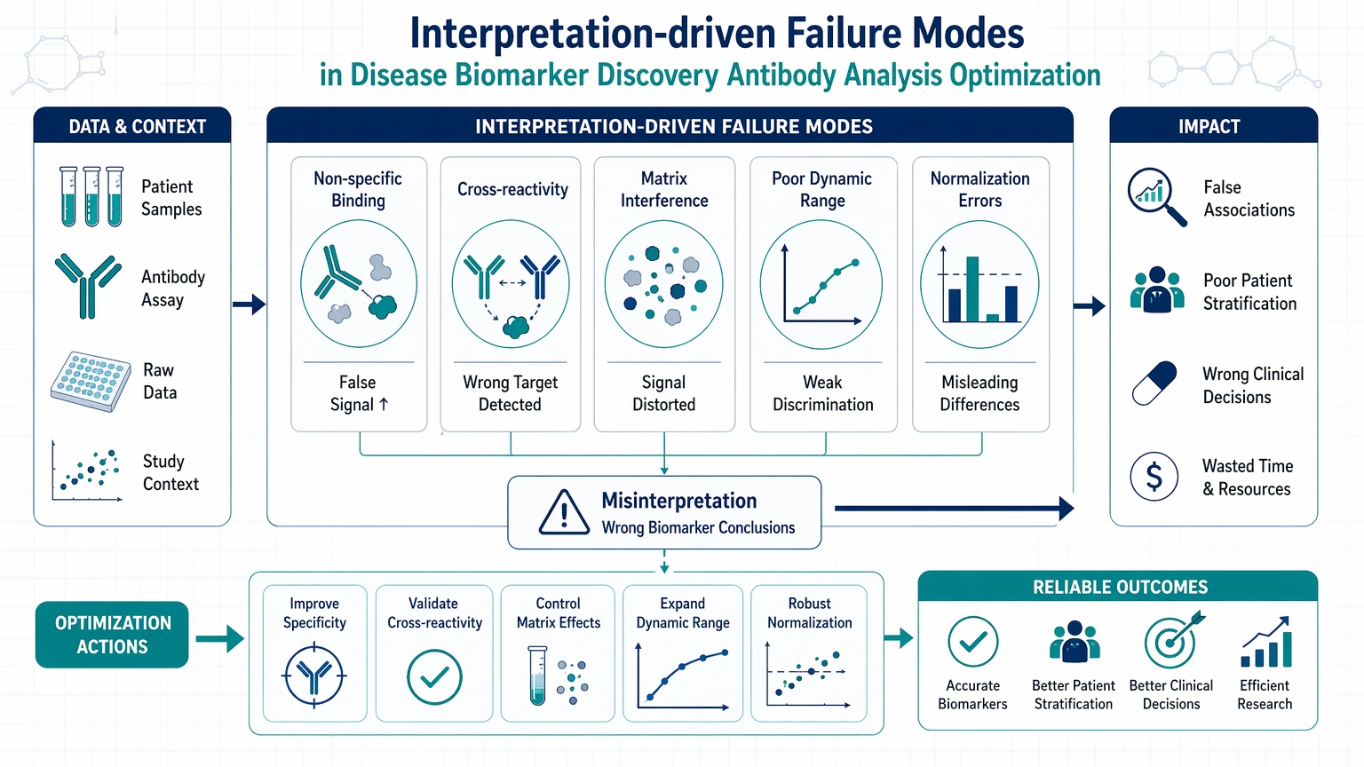
Examples include:
- signal normalization changes the candidate list substantially
- threshold rules are set after reviewing the data
- problematic replicates are averaged instead of flagged
- discovery and verification assays are compared as if they measure the same molecular event
- exploratory signal is treated as hit confirmation before orthogonal validation
These are workflow decisions rather than bench errors, and they often determine whether downstream validation succeeds.
How to Tell Whether the Problem Is Sample-, Antibody-, or Assay-Driven
A useful troubleshooting sequence starts with a simple question: does the instability follow the sample, the reagent, or the platform?
1. Check whether the pattern tracks with sample subsets
Re-plot the candidate biomarker signal by cohort, collection batch, storage history, disease subgroup, and preparation method. If one subgroup drives most of the apparent difference, the issue may be biological variability or sample handling rather than assay failure.
Useful checkpoints:
- sample input consistency
- distribution overlap between groups
- dropout frequency in low-signal samples
- correlation with hemolysis, protein concentration, or total Ig content when relevant
- concordance across technical replicates within the same sample
If the sample-level pattern explains most of the variation, changing the antibody panel alone is unlikely to fix the dataset.
2. Test whether the signal is clone-dependent or epitope-dependent
If a candidate behaves differently across antibodies, the team should ask whether the biology differs by epitope context or whether one reagent has lower specificity. Epitope accessibility can shift with denaturation state, complex formation, cleavage, glycosylation, or matrix binding.
Useful checkpoints:
- agreement across antibody clones
- signal behavior after dilution or alternate sample treatment
- expected versus observed molecular size in orthogonal protein analysis
- competition or blocking behavior, where appropriate
- specificity confirmation status from independent evidence
A clone-dependent result can still be informative, but only if the team understands which molecular form each antibody is detecting.
3. Determine whether the assay is operating near its lower analytical boundary
Low-confidence signals often cluster near the lower end of assay sensitivity. In that region, small technical shifts can create large interpretive differences.
Useful checkpoints:
- signal-to-background ratio
- coefficient of variation (CV) across replicates
- intra-assay and inter-assay variability
- limit of detection or limit of quantitation, when defined
- dilution linearity and standard-curve behavior
- batch-to-batch consistency
If candidate signals are concentrated in the least stable part of the assay, the next step may be selective re-optimization or orthogonal confirmation rather than broader screening.
4. Compare normalization choices before accepting hit ranking
If hit lists change sharply after signal normalization, the workflow may be overly sensitive to data-handling assumptions.
Review:
- blank subtraction rules
- housekeeping or total-protein normalization logic
- plate-wise versus global normalization
- threshold setting for weak positives
- outlier treatment
- replicate aggregation method
A candidate biomarker that remains stable across reasonable normalization choices deserves more confidence than one that survives only under a single processing path.
A Practical Optimization Framework for Better Interpretability
Step 1: Stabilize the sample layer before repeating assays
Do not rerun the assay immediately if sample comparability is uncertain. First standardize what can still be controlled:
- match input amount and preparation workflow as closely as possible
- separate discovery cohorts from obvious exploratory outliers
- document storage conditions and freeze-thaw exposure
- assess whether matrix effect differs across sample types
- reserve a small bridge set of representative samples for repeat testing
This step helps determine whether the candidate biomarker looks unstable because of the disease model or because the samples entering the assay are not comparable enough for reliable ranking.
Step 2: Reassess antibody selection with specificity in mind
For disease biomarker discovery antibody analysis optimization, antibody choice is not just a procurement decision. It shapes what biological claim the data can reasonably support.
Focus on:
- whether the antibody matches the relevant species, matrix, and assay format
- whether epitope accessibility is likely to differ between native and denatured conditions
- whether related proteins or isoforms create cross-reactivity risk
- whether background signal increases in complex matrices
- whether the observed signal fits known molecular context well enough for protein-level verification planning
If specificity remains uncertain, the team should lower confidence in absolute abundance interpretation and move orthogonal validation earlier in the workflow.
Step 3: Improve assay window and reduce background
Once the sample and antibody logic are clearer, optimize assay performance at the point where signal quality is actually failing.
Common fixes include:
- adjusting dilution strategy to reduce matrix interference
- narrowing the working range to the most linear part of the assay
- replacing thresholds based only on raw intensity
- strengthening control placement across plates and runs
- using targeted controls to separate true low signal from nonspecific binding
The objective is not simply to increase signal intensity. The objective is to improve analytical specificity and make weak-positive calls easier to defend.
Step 4: Use metrics to drive decisions, not just reporting
Teams often collect analytical metrics but do not use them to decide what to repeat, what to drop, and what to escalate.
For each candidate biomarker, ask:
- Is the signal-to-background ratio high enough to support ranking?
- Are replicate reproducibility and CV acceptable for the current research stage?
- Does dynamic range support separation between biological groups?
- Does dilution linearity support quantitative interpretation?
- Does the standard curve behave consistently across runs?
- Is the signal robust to normalization choices?
- Is there evidence of batch effect that changes the conclusion?
A candidate that looks statistically interesting but fails these checkpoints may still be worth mechanistic follow-up, but it should not be treated as verification-ready.
Step 5: Align discovery assays with downstream verification
Many projects stall because discovery and verification stages ask different analytical questions. A multiplex screen may detect relative shifts, while a later immunoassay expects cleaner target specificity. A western blot may provide molecular-weight context but not cohort-scale ranking. An immunoprecipitation workflow may enrich complexes rather than the exact analyte later used for confirmation.
Before expanding validation, assign each method a clear role:
- discovery assay: broad screening and initial prioritization
- verification assay: focused retesting under tighter controls
- orthogonal validation: independent support for target identity or abundance trend
- result validation: evidence that the hit is reproducible enough to justify more resources
This alignment reduces the risk of calling method disagreement a failure when the assays are capturing different aspects of the same biology.
If your team is deciding whether to reanalyze the current dataset, redesign the antibody strategy, or move selected hits into orthogonal confirmation, you can submit your requirements to MtoZ Biolabs for a focused project review tied to assay design, matrix effects, and result-validation planning.
When Orthogonal Validation Is the Right Next Step
Orthogonal validation becomes necessary when antibody analysis cannot resolve whether a signal is biologically meaningful or analytically distorted.
Move to orthogonal confirmation when:
- the same candidate biomarker changes direction across assay formats
- replicate reproducibility is acceptable but specificity remains unclear
- background signal is manageable, yet hit confirmation still fails
- one cohort reproduces and another does not, without a convincing sample explanation
- rank order is highly sensitive to normalization or threshold choice
- a low-abundance target sits near the assay detection boundary
Orthogonal methods do not guarantee agreement, but they can clarify the source of disagreement. They may show that the original hit reflected a related protein, a specific isoform context, a sample-preparation artifact, or a real biological effect that is visible only under one measurement mode.
That distinction matters because it changes the next decision: reanalyze the existing data, redesign the assay, replace the antibody, or stop investing in that candidate.
How External Analytical Support Can Help De-Risk Difficult Datasets
External support is most useful when a team already has data but cannot determine whether the bottleneck is biological, analytical, or workflow-related. In that situation, an outside review can help organize the evidence around antibody specificity, assay sensitivity, matrix effect, normalization strategy, and the fit between discovery observations and downstream protein-level verification.
For example, a team may ask an external partner to assess whether conflicting antibody readouts point to cross-reactivity, whether a low-signal dataset justifies another assay round, or whether selected candidates should move directly into orthogonal validation. This kind of support does not replace internal biological judgment. It helps narrow the most plausible failure modes before more validation work begins.
A Simple Decision Path Before You Repeat the Study
Use this sequence before scaling up another round of biomarker testing:
1. Recheck sample comparability Confirm that sample handling, input consistency, and subgroup structure do not already explain the pattern.
2. Review antibody behavior Determine whether specificity, cross-reactivity, or epitope accessibility could be distorting the signal.
3. Audit assay performance metrics Examine CV, signal-to-background ratio, dynamic range, dilution linearity, and batch effect.
4. Stress-test data interpretation rules Re-run hit ranking under alternative normalization and threshold assumptions.
5. Escalate only selected hits Move the most defensible candidates into orthogonal validation instead of repeating the full discovery workflow unchanged.
This sequence is often faster and more informative than repeating the same experiment with more samples but the same unresolved assumptions.
FAQ
How much replicate variability is too much for a candidate biomarker?
There is no single CV cutoff that fits every assay stage. In early discovery, moderate variability may still be acceptable if the signal-to-background ratio is strong and the direction of change is consistent across replicates and cohorts. In verification work, tighter replicate reproducibility is usually needed because ranking decisions become more consequential. A practical rule is to ask whether the observed variability changes the hit-prioritization decision. If it does, the candidate needs further analytical review before expansion.
Can a candidate biomarker still be useful if different antibodies give different answers?
Yes, but only after the disagreement is explained. Different antibodies may recognize different epitopes, conformations, complexes, cleavage products, or related proteins. That means the mismatch may reflect biology, weak antibody specificity, or both. The candidate should not be treated as confirmed until the team understands what each antibody is actually measuring and whether an orthogonal method supports the same biological direction.
What is the most common interpretation mistake after an exploratory hit fails validation?
A common mistake is treating the failed confirmation as proof that the candidate was never real. Another is repeating the same assay unchanged with a larger cohort. A better response is to identify where confidence first breaks down. If matrix effect or normalization instability is driving the discrepancy, more samples will not solve it. If biological variability is the main source of disagreement, subgroup-aware verification may be more informative than assay redesign.
Should low-abundance targets always move to a more sensitive assay?
Not automatically. A more sensitive assay can improve detectability, but it can also amplify background signal and nonspecific binding if specificity is still unresolved. Low-abundance targets should first be checked for dilution behavior, dropout pattern, batch consistency, and fit to the expected biology. If the target remains interesting after those checks, moving to a different assay format or orthogonal platform becomes a better-grounded decision.
Service Routes for Study Planning
For teams moving from method selection into execution, these service paths connect assay design, validation, and interpretation needs.
Conclusion
The most effective path for disease biomarker discovery antibody analysis optimization is to fix confidence losses in order: sample comparability, antibody specificity, assay performance, and interpretation rules. Teams should then reserve orthogonal validation for candidates that remain credible after those checks. This workflow will not eliminate uncertainty, and it will not make every exploratory hit reproducible across all sample sets. It does provide a clearer basis for deciding whether to reanalyze, redesign, narrow the candidate list, or move forward with result validation.
If your group is working through inconsistent signal, weak hit confirmation, or poor concordance across assay stages, contact us at MtoZ Biolabs to evaluate your project in the context of translational assay workflow review, antibody-analysis troubleshooting, and orthogonal confirmation planning.
How to order?