


How to Normalize Data in Label-Free Quantitative Proteomics?
- Differences in total sample loading
- Variability in LC–MS system performance (e.g., reduced chromatographic efficiency)
- Differences in ionization efficiency
- Batch effects associated with data acquisition time
- Tumor versus normal tissue comparisons → Preference for median normalization or MaxQuant LFQ intensity
- Time-course or dose-gradient experiments → Combination of TIC normalization with internal reference-based correction
- High-throughput batch analyses → Implementation of QC-based normalization and batch effect correction
- Boxplots or density plots: Assess consistency of global abundance distributions across samples
- PCA (principal component analysis): Examine sample clustering patterns and potential batch effects
- CV (coefficient of variation) distributions: Evaluate whether technical variability is reduced after normalization
- Heatmaps: Determine whether normalization enhances the interpretability of differentially expressed proteins
In label-free quantitative proteomics (LFQ), data normalization represents a fundamental step for ensuring inter-sample comparability and minimizing technical variability. In the absence of appropriate normalization, technical noise, such as differences in sample loading amounts and instrument performance drift, can obscure genuine biological variation, thereby introducing bias into the identification of differentially expressed proteins.
Why Is Normalization Necessary for Label-Free Quantitative Proteomics Data?
Label-free quantitative proteomics relies on signal intensities of peptides or proteins detected by mass spectrometry, typically represented by peak areas or MS1 intensities, to achieve relative quantification. However, during sample preparation and LC–MS analysis, multiple sources of systematic bias may be introduced, including:
Normalization aims to correct these non-biological sources of variation, thereby ensuring that measured protein abundance values are directly comparable across samples.
Common Normalization Methods for Label-Free Quantitative Proteomics
Normalization approaches for LFQ proteomics data can generally be classified into several categories, each characterized by specific assumptions, advantages, and limitations:
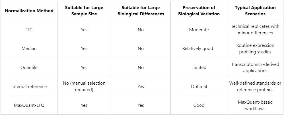
1. Total Ion Current (TIC) Normalization
(1) Principle: The total signal intensity of each sample is scaled to a common reference value (e.g., unity or the global mean), and individual protein intensities are adjusted proportionally.
(2) Advantages: Computationally simple and efficient; suitable for experiments with minimal global protein expression differences and balanced sample loading.
(3) Limitations: Less suitable for comparisons involving pronounced biological differences (e.g., tumor versus normal tissues), where systematic shifts in total protein abundance are expected.
2. Median Normalization
(1) Principle: The median protein abundance of each sample is aligned to a common reference level.
(2) Advantages: Robust to extreme values and appropriate for datasets in which only a limited number of high-abundance proteins vary substantially.
(3) Limitations: Relies on the assumption that most proteins exhibit no significant expression changes across samples.
3. Quantile Normalization
(1) Principle: Enforces identical distribution shapes of protein abundance values across all samples.
(2) Advantages: Widely applied in transcriptomics and suitable for large-scale datasets involving multiple experimental groups.
(3) Limitations: May excessively constrain biological variability and potentially distort true expression differences, particularly in highly heterogeneous samples.
4. Normalization Based on Reference Proteins or Internal Standards
(1) Principle: Protein abundance values are normalized relative to stably expressed endogenous reference proteins or exogenously added standard proteins.
(2) Advantages: More closely reflects underlying biological states when appropriate references are available.
(3) Challenges: Requires reliable identification of stably expressed proteins or the use of spike-in standards.
5. LFQ Intensity Normalization (MaxQuant-Specific)
(1) Principle: LFQ intensity values generated by MaxQuant incorporate built-in normalization procedures, including multi-level corrections based on peptide identification counts and MS1 signal intensities.
(2) Applicable scenarios: When MaxQuant is used for data processing, retaining its default LFQ normalization is generally recommended.
How to Choose an Appropriate Normalization Method for Label-Free Quantitative Proteomics Data?
Recommendations from MtoZ Biolabs:
In practical LFQ proteomics projects, normalization strategies are typically selected according to sample characteristics, experimental design, and research objectives. Representative examples include:
Quality Assessment After Normalization: Which Metrics Are Worth Attention?
Normalization alone does not guarantee data quality; systematic evaluation of normalization performance is essential for ensuring data reliability.
Commonly used quality control metrics include:
In label-free quantitative proteomics, normalization is not an optional procedure but a central determinant of data credibility. Appropriate selection of normalization strategies, combined with rigorous quality assessment, is essential for accurately capturing true biological differences among samples. Leveraging extensive experience in proteomics data analysis, MtoZ Biolabs integrates automated pipelines with manual quality control to deliver quantitative proteomics datasets characterized by high coverage, reproducibility, and traceability. For challenges related to normalization strategy selection, batch effect correction, or differential analysis, expert technical consultation can provide targeted and effective solutions.
MtoZ Biolabs, an integrated chromatography and mass spectrometry (MS) services provider.
Related Services
How to order?