





Comparative Plant Proteomics: How to Find Differential Proteins in Resistant Plants
Comparative plant proteomics finds differential proteins in resistant plants by quantifying protein abundance between resistant and susceptible materials under matched inoculation and sampling conditions, then ranking the proteins that differ consistently between those groups. The useful output is not a raw protein catalog. It is a filtered differential list, pathway context around that list, and a short set of candidates worth follow-up.
To get there, keep three conditions in place: both genotypes receive the same challenge, the same tissue is harvested at a biologically appropriate time point, and the analysis is quantitative rather than identification-only. Because the same inoculation conditions do not guarantee the same pathogen burden at harvest, disease severity should also be recorded. Without those conditions, proteins that look “resistance-related” may simply track uneven exposure, tissue mismatch, different infection stages, or late damage in the susceptible line.
What “Finding Differential Proteins” Really Means
In resistance research, “finding differential proteins” usually means answering a narrower question than people first write down. The practical question is: which proteins are higher or lower in resistant plants than in susceptible plants under the same challenge, and which of those differences are stable enough to prioritize?
Comparative plant proteomics can support that question at three layers:
- A quantitative matrix of protein abundance across resistant and susceptible samples
- A differential protein list for the resistance comparison
- Descriptive pathway context, such as GO, KEGG, database-derived protein association networks, and Reactome analysis when the species is supported
It does not, by itself, prove that any protein causes resistance. It also does not measure pathogen load, metabolite flux, or phosphorylation-level signaling unless those are planned as separate modules. Treat the differential list as ranked hypotheses, not as finished mechanism. Database-derived association networks provide functional context but do not prove direct physical interactions in the submitted samples.
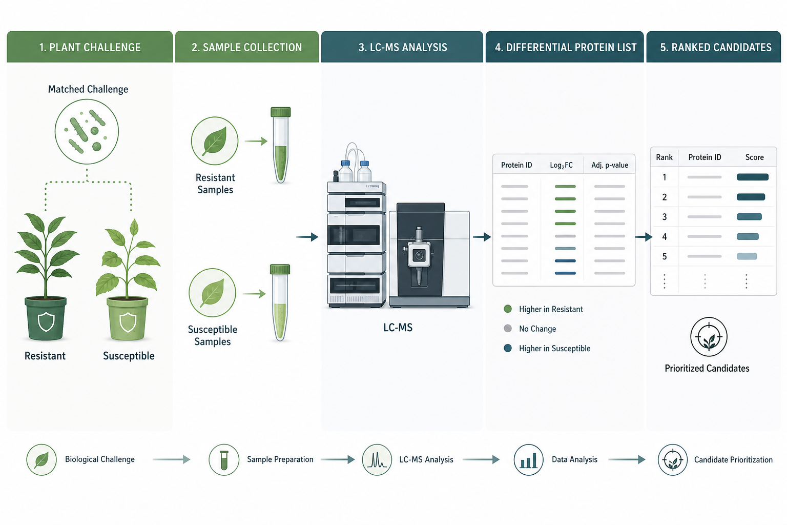
Figure 1. Matched resistant and susceptible samples feed quantitative comparison, pathway context, and candidate ranking.
Set Up the Comparison So Differential Proteins Are Interpretable
Differential proteins are only as clear as the comparison behind them. For resistant versus susceptible work, the main variable should be the plant material, while the challenge stays as steady as possible.
Define resistance with a phenotype rule you can record at harvest, such as disease score or lesion class, rather than a pedigree label alone. Give both genotypes the same inoculation dose, timing, and environment for the primary comparison. Also record disease progression and, where relevant, pathogen biomass or load, because resistant and susceptible plants may reach different infection stages even under identical treatment conditions.
Harvest the same organ, such as leaf or root, at a time point selected according to the biological process of interest. Early time points are more suitable for studying defense activation, whereas later time points may capture disease progression and tissue damage. If the best window is uncertain, a small pilot time course can be more informative than waiting only for visible symptoms.
A clean starting design is resistant challenged versus susceptible challenged. This comparison identifies proteins that differ between the two materials under challenge, but it cannot separate pre-existing genotype differences from challenge-induced resistance responses. When that distinction matters, include resistant challenged, resistant control, susceptible challenged, and susceptible control groups.
One well-characterized resistant–susceptible pair can provide a manageable discovery dataset, but the resulting proteins remain candidates associated with that specific genotype comparison. Near-isogenic materials, additional lines, or later validation can help determine whether the same candidates are more broadly linked to resistance.
Independent plants or pots usually count as biological replicates; leaves from one plant do not, if the claim is plant-level resistance. Biological replicates should be independently grown and treated experimental units. When several plants share one pot and receive treatment together, the pot may be the experimental unit.
Suggested collection amounts for planning:
|
Plant sample type |
Suggested collection amount |
|
Soft tissues such as leaves, flowers, grasses, algae, or ferns |
about 2 g |
|
Hard tissues such as roots, bark, twigs, fruits, or seeds |
about 5 g |
|
Pollen |
about 100 mg |
These are collection guides, not performance promises. Avoid degraded, contaminated, or repeatedly freeze-thawed material. Plant tissues from pathogen-challenge experiments require a biosafety and sample-handling review before submission. Samples containing viable infectious agents or presenting an unresolved biological hazard cannot be accepted. A plant proteomics project typically includes protein extraction, digestion, and LC-MS/MS. Gel imaging and similar standalone preparation work are generally outside this workflow.
How Comparative Proteomics Turns the Comparison Into Candidates
Once the sample set is realistic, choose a quantitative route. Protein identification alone can list proteins present in one condition, but it cannot reliably support abundance differences between resistant and susceptible plants.
Both DDA and DIA can support pilot and comparative studies. Method selection should consider sample complexity, required proteome depth, quantitative completeness, instrument platform, and downstream analysis goals. DIA is often considered when consistent quantification across multiple samples and reduced missing values are priorities. Common processing options include MaxQuant or Proteome Discoverer for DDA data and Spectronaut or DIA-NN for DIA data. Instruments such as Orbitrap Exploris 480, timsTOF Pro, and Orbitrap Astral can be discussed after the comparison design is clear.
A workable finding sequence looks like this:
First, quantify proteins across the resistant and susceptible groups under matched challenge.
If untreated or mock-treated controls are included, compare the challenge-induced change within each genotype before evaluating how the response differs between resistant and susceptible materials.
Next, generate the differential list for that comparison and review consistency across biological replicates. Differential proteins should be defined using a prespecified statistical workflow that considers data quality, replicate consistency, effect size, multiple-testing control, and missing-value patterns.
Then, place differential proteins into descriptive pathway context to see which defense, signaling, or metabolic themes recur.
Finally, rank a manageable candidate set for orthogonal follow-up. Priority usually rises when a protein shows statistical support, stable replicate behavior, a resistance-associated response pattern, relevance to the recorded phenotype, and practical feasibility for validation.
Candidates that differ before challenge should be distinguished from proteins that respond differently after challenge. Proteins that mainly track severe tissue damage or pathogen burden should not automatically be treated as upstream resistance regulators.
One practical habit is to keep a working shortlist that matches the available validation resources rather than trying to follow every differential hit at once. A long list looks complete, but it rarely leads to a clear next experiment. A short list tied to phenotype notes, response patterns, and pathway themes is easier to discuss with collaborators and easier to move into western blot, targeted assays, or a companion omics module.
|
Output layer |
What it helps you do |
Limit to keep in view |
|
Quantitative abundance matrix |
Compare resistant and susceptible samples |
Needs matched challenge, tissue, and timing |
|
Differential protein list |
Spot proteins associated with the resistance comparison |
May include genotype background effects |
|
Pathway and association context |
Group candidates into biological themes |
Descriptive and species-dependent |
|
Ranked candidate shortlist |
Choose proteins for follow-up |
Needs independent validation |
A first round often uses one well-matched resistant versus susceptible pair under challenge. A later expansion can add unchallenged baselines, another time point, or a small line panel once phenotype scoring and harvest timing are stable. This staged approach keeps the first dataset manageable while allowing later testing of whether the same candidates recur across additional materials.
Read the Differential List Without Overclaiming
A useful comparative proteomics report for resistant plants answers three practical points:
- Which proteins differ between resistant and susceptible groups
- Which pathway themes those proteins point to at a descriptive level
- Which candidates are realistic to validate next
It does not answer whether a protein is sufficient for resistance, whether pathogen growth was blocked by that protein, or whether a pathway flux changed. Those conclusions need separate functional or metabolite work.
Common reading mistakes are easy to avoid. Do not treat a late susceptible collapse sample as a clean resistance contrast. Do not merge unchallenged and challenged plants into one resistant group. Do not promote a pathway enrichment hit into a mechanism claim before validation. Keep phenotype notes beside the differential list so candidates that track a clear resistance score rise above proteins linked only to uneven disease progress.
During interpretation, distinguish proteins that differ constitutively between genotypes from proteins that respond to challenge in both materials and proteins whose challenge response differs between resistant and susceptible plants. The last category is often more informative when the goal is to investigate resistance-associated responses.
If early defense signaling is the next question after an abundance screen, plant phosphoproteomics can be planned as a companion study. If defense metabolites matter, plant metabolomics is a better follow-up than inferring metabolite change from protein data alone.
When several resistant lines or cultivars are available, resist the urge to compare all of them in the first round. One well-scored pair under matched challenge usually produces a more manageable discovery dataset, although it does not eliminate genetic-background effects. After that list is stable, a later panel can test whether the same candidates recur across related resistant materials. That sequence protects interpretation and keeps sample demand manageable.
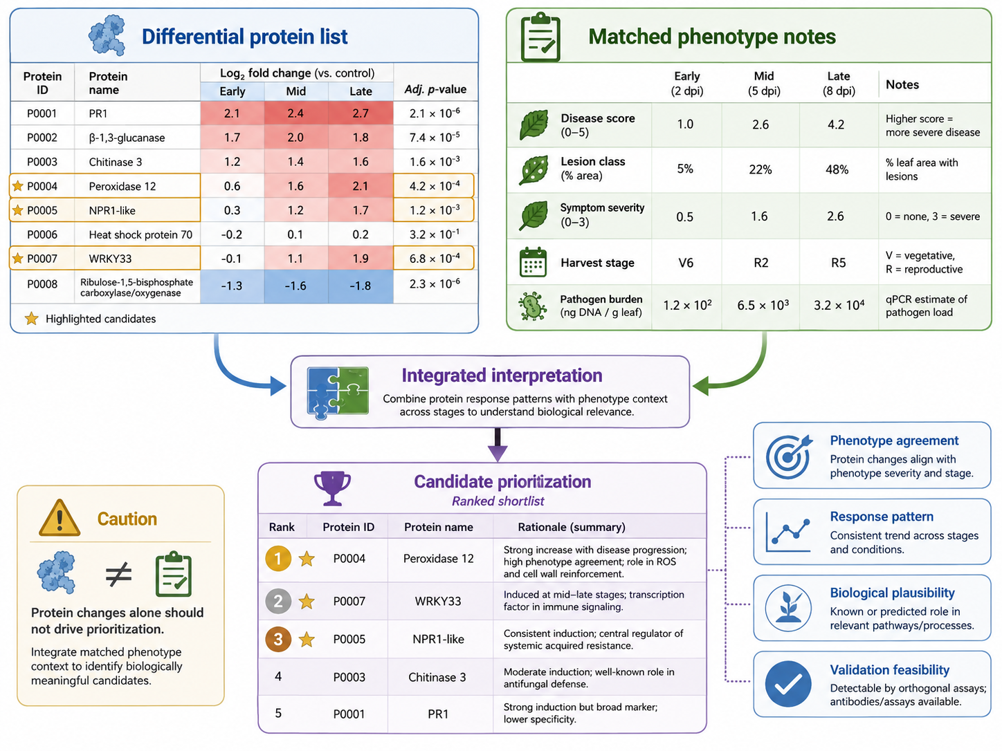
Figure 2. Pair the differential protein list with matched phenotype notes before prioritizing candidates.
Before You Start Looking for Candidates
Write the resistance comparison in one sentence, including genotype pair and challenge.
Confirm both materials receive the same exposure and that the same tissue will be harvested.
Decide whether the goal is to identify differences under challenge or resistance-associated challenge responses.
Include untreated or mock-treated controls when genotype background must be separated from challenge response.
Choose the harvest time according to whether the project targets early defense, intermediate response, or later disease progression.
Plan how disease severity and, where relevant, pathogen load will be recorded.
Plan collection amounts for the chosen tissue and keep biological replicates independent.
Choose quantitative comparison rather than identification-only when abundance differences are the goal.
Decide how candidates will be ranked and what follow-up module comes next.
If these points are still open, settle them before harvest. MtoZ Biolabs can review the genotype pair, scoring rule, tissue, challenge timing, control design, replicate structure, and expected differential output before the analytical plan is finalized.
Related Services
Plant Phosphoproteomics Analysis Service
Frequently Asked Questions
1. How does comparative plant proteomics find differential proteins in resistant plants?
It quantifies proteins in resistant and susceptible materials under matched challenge conditions, then ranks proteins that differ consistently between those groups and places them in pathway context. With untreated controls, it can also help separate genotype background from challenge-associated responses.
2. Is protein identification enough?
No, not for abundance differences. Identification lists proteins present in a sample. Finding differential proteins requires quantitative comparison.
3. Can differential proteins prove a resistance mechanism?
No. They are ranked candidates associated with the resistance comparison. Functional validation is still required.
4. Are untreated controls needed?
They are recommended when the goal is to distinguish pre-existing genotype differences from challenge-induced resistance responses. A challenged-only comparison cannot make that distinction.
5. How much tissue should be planned?
As a practical guide, soft tissues are often collected at about 2 g, hard tissues at about 5 g, and pollen at about 100 mg per biological replicate. Confirm unusual sample types before harvest.
6. Should both genotypes receive the same challenge?
Yes for the main resistance comparison. Use matched inoculation conditions, but also record disease severity because infection progress may still differ between resistant and susceptible plants.
7. What should be shared before the project starts?
Share the genotype pair, resistance scoring rule, tissue type, challenge protocol with timing, planned groups and replicates, proposed harvest time and control design, and the expected differential output.
Conclusion
Finding differential proteins in resistant plants is a comparative, quantitative task. Keep the inoculation conditions and tissue matched, choose the harvest time according to the biological stage of interest, quantify abundance across resistant and susceptible groups, and read the differential list together with pathway context, challenge-response patterns, and phenotype notes.
A challenged resistant-versus-susceptible comparison identifies proteins that differ under challenge, whereas a four-group design can better distinguish genotype background from resistance-associated responses. Use that shortlist to guide follow-up, not to declare mechanism.
To review a comparative plant proteomics plan aimed at differential proteins, contact MtoZ Biolabs with the genotype pair, scoring rule, tissue, challenge scheme, groups, sampling time and control design, and expected output.
How to order?