



Protein interaction networks from proteomic mass spectrometry are assembled after the identification table is filtered, scored, and typed. A raw LC-MS/MS list from AP-MS, IP-MS, or proximity labeling reports proteins present in that digest. It does not report edges. Nodes enter the graph only after bait recovery and control subtraction. Edges receive a stated evidence score, such as enrichment versus empty-tag, IgG, or empty-enzyme tubes. Node relationships must be typed: bait-prey spokes are the default, prey-prey lines are not automatic, and multi-bait overlap is a separate claim. Gene-set enrichment and a network figure then describe the ranked set. They do not convert leftover identifications into a finished interactome.
Researchers who already have bait captures, matched controls, and a written network claim can review MtoZ Biolabs MS-Based Protein-Protein Interaction Analysis Service for feasibility. Pair-level method choice after a shortlist is covered in Measuring Protein-Protein Interactions.
Proteomic Identifications Are Inputs, Not Networks
The first output of interaction proteomics is a protein table. MaxQuant against UniProt or a client FASTA assigns accessions and intensities. Identification depth is typically hundreds to thousands of proteins and depends on the sample. That count is digest inventory, not network size.
Published AP-MS maps that later appear as graphs were built from scored enrichments, not from unfiltered names (Huttlin et al. 2015). Co-enrichment and proximity can still be indirect (Hein et al. 2015). A bridging subunit, a shared-organelle contaminant, and a true neighbor can occupy the same row.
Do not treat peptide identification as interaction inference. MS/MS assigns sequences. Interaction status is added later by controls, scores, and a relation rule. Generic ionization lectures do not move a table toward protein interaction networks.
If the bait is missing from the bait capture, stop. No graph should be drawn from a run that did not recover the intended protein. Product-level digest choices for already-run IPs are covered in Cellular IP Product Mass Spectrometry Detection.
The comparison below keeps an unfiltered identification table and a scored graph on separate tracks.
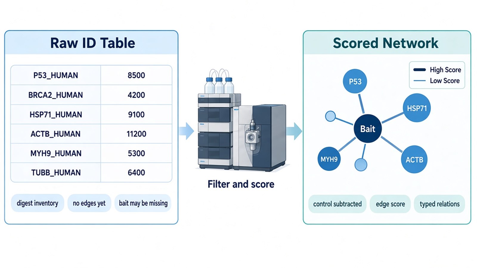
Figure 1. Identification Table vs Filtered and Scored Interaction Network.
Protein Filtering Before Nodes Are Kept
Protein filtering decides which accessions are allowed to become nodes. Keep the bait if it was recovered. Remove or annotate proteins that are equal in the matched control. Empty-tag and bead-only tubes serve tagged AP-MS. Isotype IgG or bead-only tubes serve antibody IP-MS. Empty-enzyme and no-substrate arms serve proximity labeling. The IP-Mass Spectrometry Service and Proximity Labeling Mass Spectrometry paths use different control geometries, but both require the comparison before a name is plotted.
Recurrent-contaminant catalogs such as the CRAPome help interpret leftovers after experimental subtraction (Mellacheruvu et al. 2013). They do not replace the matched control. Antibody chains, keratins, and trypsin are expected reagent or handling proteins. Label them. Do not promote them as novel partners.
Do not filter by protein class alone. Ribosomal and cytoskeletal names are frequent background, yet some baits sit in those complexes. Relative intensity versus the control tube decides whether the name stays a candidate. Co-IP-MS-specific background and replicate checks are expanded in Co-IP MS: Decoding the Construction of Protein Interaction Networks.
Write the keep-or-drop rule before search. Changing the cutoff after favorite names appear is not a second experiment.
Edge Evidence Scoring After the Filter
An edge needs a stated score, not only a remaining accession. The usual experimental score is enrichment versus the matched control set. Fold change or intensity ratio is usable when the control design is clean. SAINT ranks bait captures against controls when replicates exist (Choi et al. 2011). Spectral-count difference is a third number. Do not mix the three on one color scale without a legend.
High score still means co-enriched or proximal under the submitted wash or labeling window. It does not mean direct binding. Orthogonal pair tests stay a later step when a named pair must be examined outside the original lysate.
State the score type in the notebook before the graph is exported. A SAINT probability of 0.9 and a two-fold intensity ratio are not interchangeable ranks. Names that fail the written threshold stay off the first protein interaction networks figure.
Do not convert a screen intensity into a binding constant. Affinity belongs on a prepared pair, not on a proteomic rank.
Node Relationships in Bait-Centered and Multi-Bait Graphs
Node relationship is the sentence an edge is allowed to support. The default AP-MS, IP-MS, or proximity graph is a spoke: bait to each passing prey. Two preys in one bait table are not automatically connected to each other. Shared appearance can reflect one complex, two complexes on the same bait, or shared background.
Multi-bait overlap is a different relation. A prey recovered with two baits can support a shared-complex hypothesis when both captures passed their own controls. It still does not prove that the two baits touch. Reciprocal capture, where A recovers B and B recovers A, is a third relation and requires a second IP.
Database resources can annotate a filtered experimental set. They should not import first neighbors that this capture never recovered. Overlay nodes need a different symbol from experimental nodes if both appear on one canvas.
Do not collapse spoke, prey-prey, multi-bait, reciprocal, and database overlay into one unlabeled line type. The table below is a relation rule for protein interaction networks, not a ranking of software.
Object |
Allowed relation |
Not an automatic edge |
|---|---|---|
Raw ID in the bait digest |
Presence in that run |
Bait-prey or prey-prey contact |
Enriched vs matched control |
Spoke from bait to that prey |
Direct binding |
Two preys in one bait table |
Two spokes to the same bait |
A prey-prey edge |
Prey seen with two passing baits |
Shared-complex hypothesis |
Contact between the two baits |
GO or pathway term on the filtered set |
Annotation of that set |
A new experimental edge |
Public-database neighbor |
Prior or transferred context |
A measured edge in this study |
The table is a construction rule. Visualization must keep those types visible.
Enrichment Analysis and Result Visualization
Enrichment analysis asks whether a stated gene set is over-represented for Gene Ontology or pathway terms versus a stated background (Ashburner et al. 2000). For protein interaction networks, the input must be the filtered, scored candidate set. Running enrichment on the raw identification list mainly rediscovers abundant and reagent proteins.
State the background. Common choices are the proteins identified in the same experiment or a taxon-wide list. The two backgrounds change the same term list. Enrichment describes annotation of the kept nodes. It does not create edges and does not replace edge scoring.
Centrality metrics on the figure are display properties of the drawn graph. Degree or betweenness on an unfiltered ID list is not a target-discovery result. Do not convert a hub rank into a therapeutic claim.
Visualization is a display of the ranked table. Node size can encode bait-normalized intensity. Edge weight can encode the stated score. Color can encode relation type or replicate support. A network viewer can render that table. The figure remains a candidate map.
Stage |
Question |
Required input |
Typical output |
|---|---|---|---|
Protein filter |
Which accessions may become nodes? |
Bait recovery plus matched controls |
Kept candidate table |
Edge scoring |
How strong is each bait-prey claim? |
Intensity or SAINT versus controls |
Ranked spoke list |
Relation typing |
What sentence does each line support? |
Single-bait or multi-bait design |
Labeled edge types |
Enrichment |
Which annotations are over-represented? |
Filtered set plus a stated background |
Term table, not new edges |
Visualization |
How is the ranked set shown? |
Score, origin, and relation legend |
Candidate network figure |
The table is a data-flow rule, not a menu of optional extras.
Ship the bait, control arms, replicate plan, intended relation types, and whether enrichment will use the filtered set only. For a full capture-to-search workflow, the usual starting point is a client-supplied IP-grade antibody or a tagged sample, plus cells or tissue that express the bait. Vector construction, overexpression, and knockout are outside Co-IP or AP-MS intake. Planning amounts for liquid IP or pull-down products are at least 20 ug total protein at more than 0.5 ug/uL, with SDS kept below 0.1 percent.
The diagram below links filter, score, relation type, enrichment set, and visualization rules to a network request.
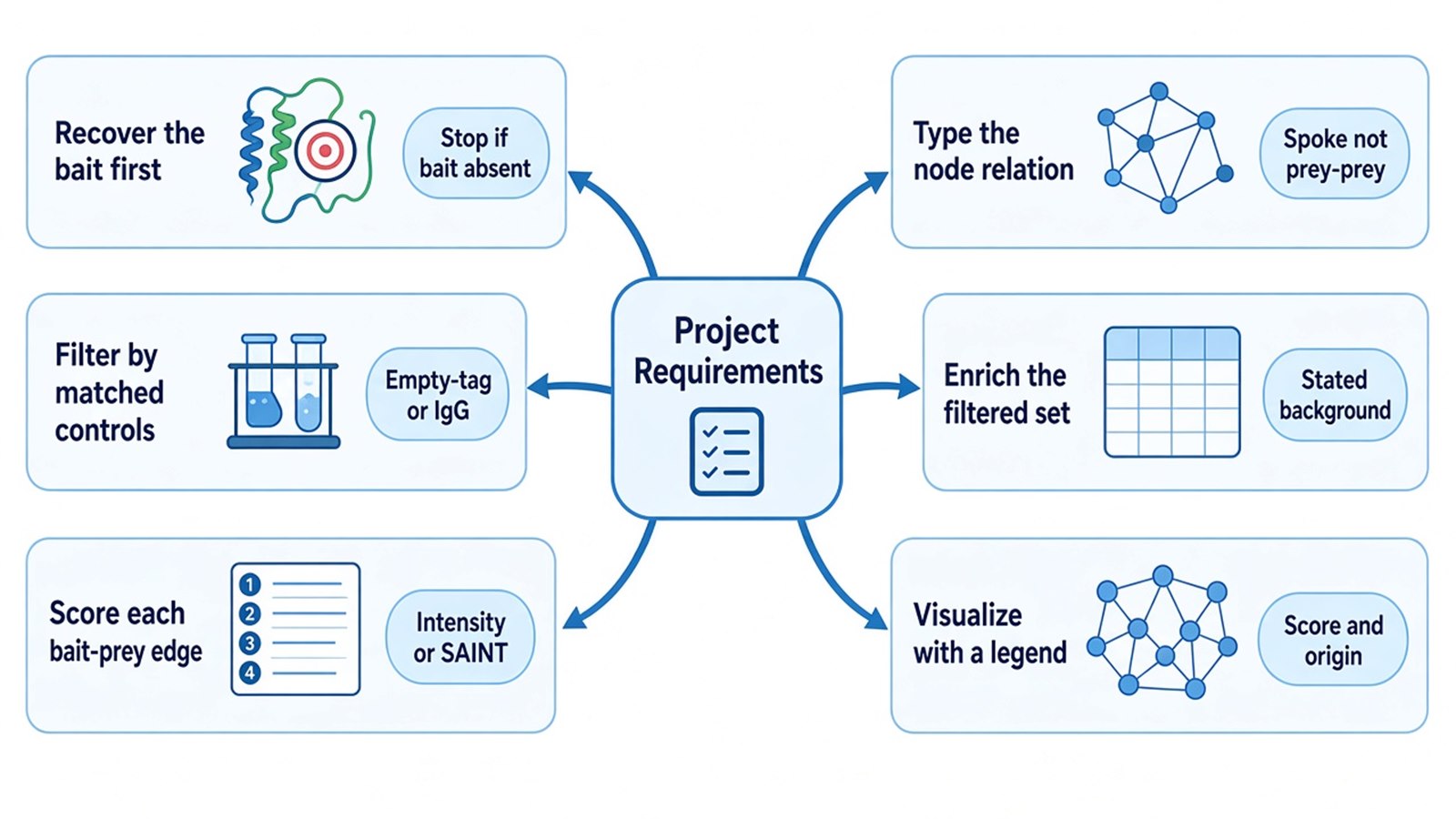
Figure 2. Matching Project Requirements With Network Data-Flow Stages.
Deliverables for construction typically include the identification table, the control-filtered candidate list, the stated edge scores, and an optional network display of that ranked set. Enrichment, if requested, is a term table on the filtered set with a stated background. Deliverables do not include a claim that every plotted line is a direct cellular binder, a guaranteed node count, or a certificate that imported database edges were measured here. Intake for mixed capture designs can also be reviewed under Protein-Protein Interaction Analysis. To start, send the bait, controls, intended relation types, and reserved figure claim to info@MtoZ-Biolabs.com or use the site inquiry form so the data flow can be split before work starts.
Frequently Asked Questions
1. Can GO enrichment of the raw identification list replace edge scoring?
No. Enrichment annotates a gene set. Edge scoring ranks bait-prey evidence versus controls. Run enrichment only after the candidate table is filtered, and keep the two tables separate.
2. When may two preys in one AP-MS table be drawn as a prey-prey edge?
Only when a second experiment supports that pair, such as reciprocal IP, a defined-pair pull-down, or a stated multi-bait overlap rule. Shared presence in one bait digest is not enough.
3. Should node centrality on the first figure become the follow-up target list?
Not by default. Centrality describes the drawn graph. Follow-up targets should come from enrichment score, replicate support, and the reserved pair assay, not from hub rank on an unfiltered list.
4. Can AP-MS and proximity lists be merged into one edge table?
They can be shown on one canvas if each edge keeps its method tag and its own control rule. Do not collapse a co-purification score and a biotinylation score into one unlabeled weight.
5. What should a feasibility email attach when the request is a network plus enrichment?
Attach bait and control plans, the keep-or-drop rule, the score type, the allowed relation types, and the enrichment background. Feasibility review will treat the figure as a display of a filtered table.
Researchers can keep protein interaction networks as a scored, typed graph of proteomic mass spectrometry candidates, then confirm bait, controls, and display rules through MtoZ Biolabs MS-Based Protein-Protein Interaction Analysis Service.
Reference
- E.L. Huttlin, L. Ting, R.J. Bruckner, F. Gebreab, M.P. Gygi, J. Szpyt, S. Tam, G. Zarraga, G. Colby, K. Baltier, et al. (2015). The BioPlex Network: A Systematic Exploration of the Human Interactome. Cell, 162, 425-440. https://doi.org/10.1016/j.cell.2015.06.043
- M.Y. Hein, N.C. Hubner, I. Poser, J. Cox, N. Nagaraj, Y. Toyoda, I.A. Gak, I. Weisswange, J. Mansfeld, F. Buchholz, et al. (2015). A human interactome in three quantitative dimensions organized by stoichiometries and abundances. Cell, 163, 712-723. https://doi.org/10.1016/j.cell.2015.09.053
- D. Mellacheruvu, Z. Wright, A.L. Couzens, J.P. Lambert, N.A. St-Denis, T. Li, Y.V. Miteva, S. Hauri, M.E. Sardiu, T.Y. Low, et al. (2013). The CRAPome: a contaminant repository for affinity purification-mass spectrometry data. Nat. Methods, 10, 730-736. https://doi.org/10.1038/nmeth.2557
- H. Choi, B. Larsen, Z.Y. Lin, A. Breitkreutz, D. Mellacheruvu, D. Fermin, Z.S. Qin, M. Tyers, A.C. Gingras, A.I. Nesvizhskii (2011). SAINT: probabilistic scoring of affinity purification-mass spectrometry data. Nat. Methods, 8, 70-73. https://doi.org/10.1038/nmeth.1541
- M. Ashburner, C.A. Ball, J.A. Blake, D. Botstein, H. Butler, J.M. Cherry, A.P. Davis, K. Dolinski, S.S. Dwight, J.T. Eppig, et al. (2000). Gene ontology: tool for the unification of biology. Nat. Genet., 25, 25-29. https://doi.org/10.1038/75556
