Biolayer interferometry data analysis starts after association and dissociation traces exist, not after a description of optical interference. The sensor records a nanometer-scale shift as analyte binds a ligand on the tip. That raw curve is not a rate constant. Baseline alignment and reference subtraction come first. A 1:1 model is fitted next, usually across a concentration series. ka, kd, and KD are reported only after residuals are inspected. A fitted KD belongs to the prepared pair, the loading density, and the buffer used in that run. Reference sensors and a concentration series belong in the same plan. It is not the cellular affinity, and it is not a functional outcome.

Researchers who already have purified ligand and analyte, a planned immobilization handle, and a written kinetic claim can review the MtoZ Biolabs Biolayer Interferometry (BLI) Service for feasibility. Method-level choice among pair assays is covered in Measuring Protein-Protein Interactions.

Raw Traces Are Not Kinetic Constants

A BLI trace has a loading segment, a baseline, an association window, and a dissociation window. Data analysis assigns those windows before any model is opened. Ligand loading must be stable enough that later association is not a continuation of immobilization drift. A dipping sensor does not use continuous microfluidic flow. Stirring and well-to-well steps replace an SPR-style flow cell, so interstep jumps must be inspected rather than ignored.

Do not convert a single-concentration nanometer shift into KD. Equilibrium height still depends on active ligand, analyte activity, and nonspecific binding to the tip. Competitive or tandem-tip designs can ask whether two analytes block one another. Those designs are separate from a 1:1 kinetic report and should not be mixed into the same fitted file.

If the next sentence must be a higher-sensitivity kinetic constant on a scarce or low-mass analyte, move the pair to the Surface Plasmon Resonance Technology service rather than force a noisy BLI curve.

Baseline Alignment and Reference Subtraction

BLI data analysis subtracts two backgrounds before fitting. A reference sensor carries no ligand, or carries an irrelevant protein on the same chemistry. That sensor measures bulk shift and sticky binding to the matrix. A reference well contains buffer without analyte. Subtracting both, often called double referencing, leaves the ligand-dependent association and dissociation.

Align the y-axis to the pre-association baseline so a concentration series starts together. Align the x-axis to the start of association. Correct interstep offsets when a tip moves between wells and the jump is mechanical rather than binding. Do not subtract a drifting reference that itself binds analyte. Do not hide a rising baseline inside a smoother and then fit the smoothed file as if it were raw.

Bulk refractive-index steps that remain after double referencing are a buffer mismatch, not a kinetic phase. Match salt, glycerol, and detergent between analyte and baseline wells. Boundary planning avoids DTT, beta-mercaptoethanol, glycerol, detergent, and salt above 200 mM unless the same matrix is present in every well and still allows a flat baseline.

The comparison below keeps preprocessing and the later 1:1 fit on separate tracks.

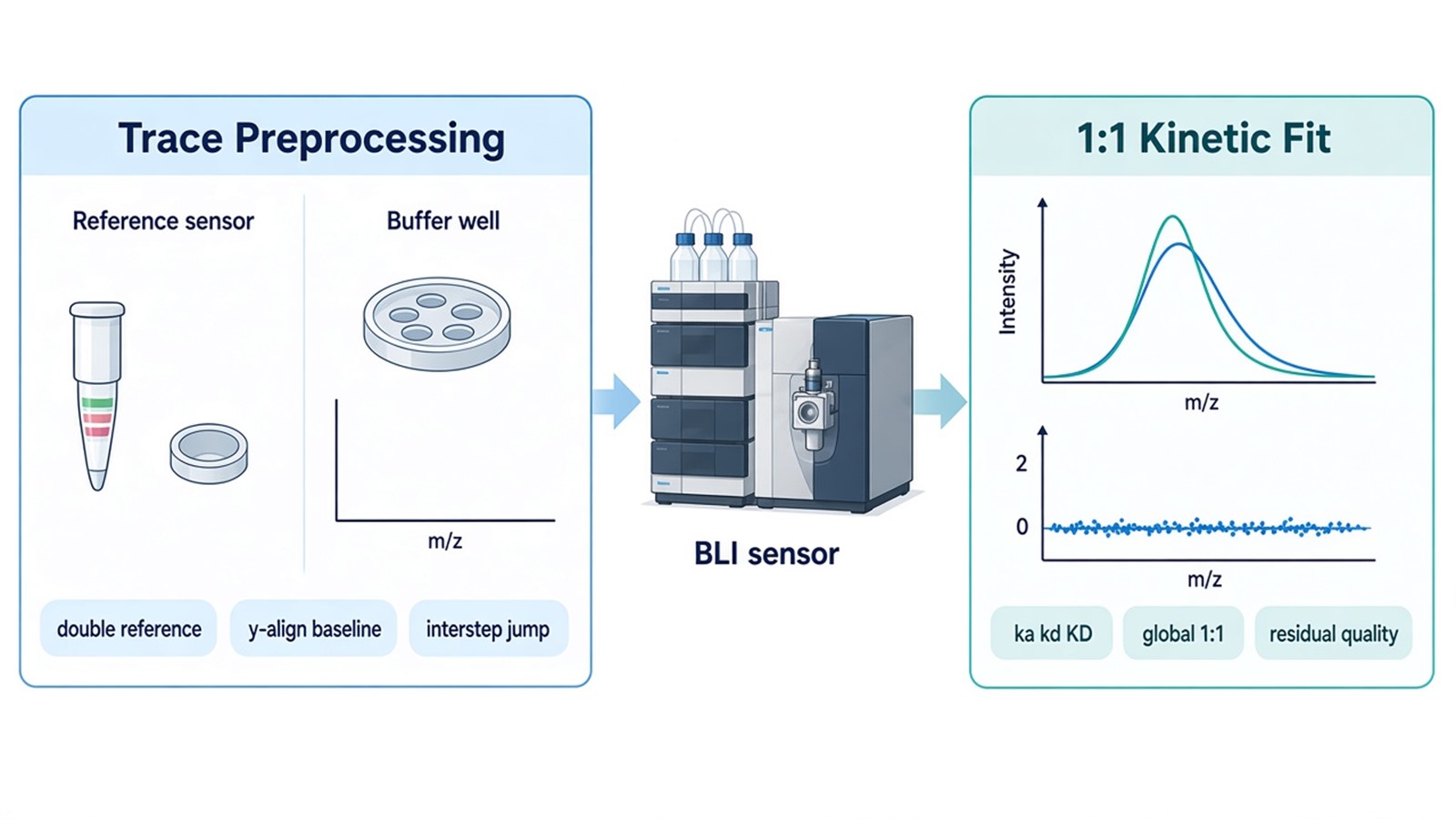
Figure 1. BLI Trace Preprocessing vs 1:1 Kinetic Fitting.

Fitting a 1:1 Model Across a Concentration Series

BLI data analysis uses a 1:1 Langmuir model when one analyte binds one immobilized site without cooperativity. Association is governed by ka and the free analyte concentration. Dissociation is governed by kd. KD is kd divided by ka. Global fitting shares ka and kd across the series and lets Rmax vary with loading when that is the experimental design (Concepcion et al. 2009; Sultana and Lee 2015).

Use at least three, and preferably five or more, analyte concentrations that span the expected KD. A single well can show binding. It cannot separate ka from kd with the same confidence as a series. Local fits to one curve are diagnostics. They are not the reported global constants.

Octet BLI Analysis, or an equivalent disclosed package, can run the 1:1 model. Software convergence is not acceptance. A bivalent antibody, a dense streptavidin surface, or an aggregated analyte can still return a number. That number is then an apparent constant, not a 1:1 mechanism.

Do not start from a 2:1 or mass-transport model just to improve the overlay. First ask whether loading was too high, whether the analyte is oligomeric, or whether the pair should move to SPR.

Judging ka, kd, KD, and Residual Quality

Residual quality decides whether BLI data analysis can write the 1:1 constants. Plot observed minus fitted signal against time. Accepted residuals scatter around zero without a smile, a lag at the association start, or a slow leftover during dissociation. Systematic curvature means the model missed a second phase.

Rmax should be consistent with the loaded ligand and should not explode to absorb a bad shape. ka that hits the upper software bound, or kd that is slower than the recorded dissociation window, should be flagged. KD reported without the parent ka and kd hides those failures.

A fitted KD is a biosensor value. Different immobilization, activity, or method can shift the number, and affinity methods can disagree widely on the same pair. The constant should stay attached to the sensor chemistry and the buffer. It should not be restated as occupancy in a cell or as functional regulation.

Analysis item	What is inspected	Accepted use	Not accepted as
Double-reference subtraction	No-ligand sensor and buffer well	Ligand-dependent trace	A KD from the raw nm shift
Baseline and interstep align	Pre-association zero and well jumps	Overlay of a concentration series	Proof of a 1:1 mechanism
Global 1:1 fit	Shared ka and kd across wells	Reported ka, kd, and KD	Cellular affinity
Residual plot	Random versus curved leftover	Pass or reject the 1:1 model	License to treat a bivalent surface as 1:1
Rmax and window	Loading consistency and recorded time	Plausible amplitude and rates	A constant at the software bound

The table is an acceptance rule, not a ranking of sensor chemistries.

When the Fit Should Stop, and How Samples Should Arrive

Stop a 1:1 report when residuals stay curved after loading is lowered, when the analyte is clearly multivalent, or when the signal is near the noise of a small molecule. Weak pairs and low-mass analytes are a documented BLI limit. Scarce samples that need higher sensitivity should transfer to SPR rather than be averaged into a forced fit.

Epitope binning or tandem blocking is a different report. It can use the same instrument. It should not reuse a failed 1:1 file as a competition result.

Ship purified ligand and analyte for BLI data analysis as powder or as snap-frozen solution on dry ice. State immobilization chemistry, expected activity, buffer, and the kinetic claim. Declare glycerol, detergent, reductant, and salt. Mechanism-level pair work after a named contact is also discussed in Mechanism of Protein-Protein Interaction. Intake for a broader pair menu can start from Protein-Protein Interaction Analysis.

The diagram below links referencing, the concentration series, residual checks, and the SPR transfer rule to a BLI request.

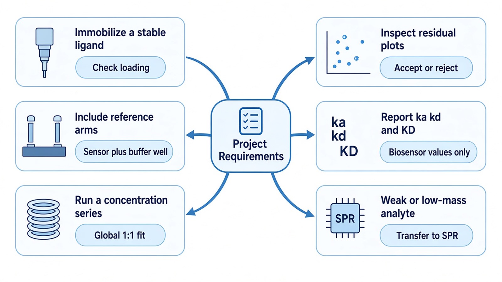
Figure 2. Matching Project Requirements With BLI Data Analysis.

Deliverables typically include referenced traces, the global 1:1 overlay, ka, kd, KD, residual plots, and a short methods note on sensor type and windows. Deliverables do not include a cellular KD, a unique binding pose, or a claim that a converged fit proves a 1:1 mechanism when residuals are curved. To start intake, send the pair, handles, buffer, planned concentrations, and the intended kinetic sentence to info@MtoZ-Biolabs.com or use the site inquiry form so the analysis path can be confirmed before shipment.

Frequently Asked Questions

1. Is a single-concentration nanometer shift enough for BLI data analysis to report KD?

No. One well can show binding. KD from a 1:1 kinetic model needs a concentration series, referenced traces, and residuals that support shared ka and kd.

2. When should a converged 1:1 fit still be rejected?

Reject the 1:1 report when residuals are systematically curved, when Rmax is implausible for the loading, or when ka or kd sits on a software bound. A second model is not the first fix.

3. When should the pair move to SPR instead of another BLI fit?

Move to SPR when the analyte is low mass or weakly bound, when the BLI signal sits near noise, or when sample amount is limited and higher sensitivity is required.

4. Can glycerol or detergent stay in the analyte if the ligand loaded well?

Only if the same matrix is in the baseline wells and the referenced trace stays flat. Those additives are otherwise avoided because they create bulk steps that look like binding.

5. Does a fitted BLI KD equal the affinity in cells?

No. The constant belongs to the prepared pair on that sensor. It should not be rewritten as cellular occupancy or as a functional effect.

Researchers can keep preprocessing, 1:1 fitting, and residual review as three sequential checks, then confirm ligand, analyte, and the kinetic claim through the MtoZ Biolabs Biolayer Interferometry (BLI) Service.

Reference

1. J. Concepcion, K. Witte, C. Wartchow, et al. (2009). Label-free detection of biomolecular interactions using BioLayer interferometry for kinetic characterization. Comb. Chem. High Throughput Screen., 12, 791-800. https://doi.org/10.2174/138620709789104915
2. A. Sultana, J.E. Lee (2015). Measuring protein-protein and protein-nucleic acid interactions by biolayer interferometry. Curr. Protoc. Protein Sci., 79, 19.25.1-19.25.26. https://doi.org/10.1002/0471140864.ps1925s79